What happens when you have missing data? Many people recommend using multiple imputation (see Briggs et al. 2003; Faria et al. 2014; Gomes et al. 2013; Hunter et al., 2015; Hughes et al., 2016). This approach, however, generally assumes that data are missing at random. Missing at random could be interpreted as the probability that health outcomes that are observed in the data are independent of their true value, conditional on the fully
observed data (selection perspective); an alternative perspective would be that “given the fully observed data, the distribution of potentially missing data does not depend on whether those data are observed (pattern‐mixture
perspective).”
But what happens if missing data points are not random, but rather provide some information on the censoring process? For instance, if you measure changes in patient quality of life from baseline, it could be the case that the patients whose quality of life declines the most are least likely to respond to a survey. A paper by Mason et al. (2018) proposes a Bayesian approach for dealing with data that are missing not at random. Their approach relies on 6 steps:
- Use previous studies and expert opinion to assess the extent and causes of missing data. Identify variables that predict of missing data.
- Formulate flexible Bayesian statistical model, such as a pattern-mixture model.
- In the protocol, specify plausible assumption about the missing data for the base case analysis.
- Specify the scope of sensitivity analyses for the missing data, and collect prior information from experts to inform these.
- When the data are available, perform the base case and sensitivity analysis.
- Report the results of the base case analysis, and discuss the extent to which they are robust under the sensitivity scenarios.
The authors provide a formal derivation of the math underlying these steps. They also provide an example from the IMPROVE trial, a multicenter randomized controlled trial that compared outcomes for patients ruptured abdominal
aortic aneurysm who used emergency endovascular strategy (eEVAR) against an open repair. Both treatment strategies were evaluted for clinical efficacy and cost effectiveness.
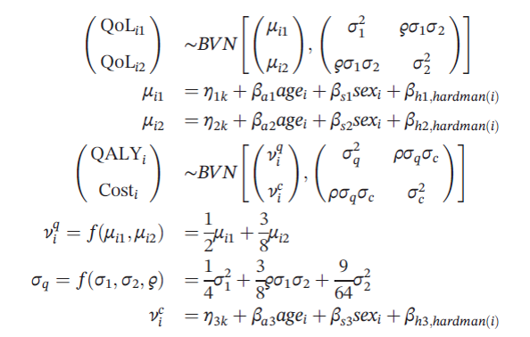
Quality of life was measured at 3 and 12 months after randomization. The statistical model is outlined below where quality of life follows a bivariate normal distribution and depends whether individual i was in treatment arm k, the patient’s age, sex, and the Hardman index, a disease‐specific morbidity score.
Using this model, the authors then define a base case that assumed that quality of life and cost outcomes were missing at random. The authors then implement their sensitivity analysis approach where:
- μij = xiTβjk + (1-Rij)Δjk
- νic = γkc + (1-Si)Γ
where Rij=1 if quality of life is observed and 0 otherwise, Si=1 is similarly defined to equal 1 if the patient’s costs is observed and 0 otherwise. The xi is a vector of covariates.
Each of the Δijk parameters represents the average (marginal) difference between the observed and missing values of QoLijk. However, the distribution implied for any individual missing value will also be influenced by the observed QoLs for that individual, through the covariance matrix Σk.
The authors create a vector of the Δijk terms and assume it is distributed multivariate normal with a variance-covariance matrix of Σk.
The question is, where do these Δijk come from? The authors claim that asking expert opinion is best. Other papers propose using the Delta Method. The delta method assumes all the Δijk are equal to zero, which is equivalent to missing at random. The sensitivity analysis then increases the vector of Δijk until the treatment is no longer cost effective. Then a research could determine the plausibility of such a missing not at random result that would cause this CEA tipping point to occur.
In short, the Mason approach is fairly flexible to be able to model missing not at random observations, but largely hinges on experts being able to determine the nature of any missing not at random result to inform the model’s priors.
Sources:
- Mason AJ, Gomes M, Grieve R, Carpenter JR. A Bayesian framework for health economic evaluation in studies with missing data. Health economics. 2018 Jul 3.
- Briggs, A., Clark, T., Wolstenholme, J., & Clarke, P. (2003). Missing …presumed at random: Cost‐analysis of incomplete data. Health Economics, 12, 377–392.
- Faria, R., Gomes, M., Epstein, D., & White, I. R. (2014). A guide to handling missing data in cost‐effectiveness analysis conducted within randomised controlled trials. PharmacoEconomics, 32, 1157–1170.
- Gomes, M., Diaz‐Ordaz, K., Grieve, R., & Kenward, M. G. (2013). Multiple imputation methods for handling missing data in cost‐effectiveness analyses that use data from hierarchical studies: An application to cluster randomized trials. Medical Decision Making, 33(8), 1051–1063.
- Hughes D, Charles J, Dawoud D, Edwards RT, Holmes E, Jones C, Parham P, Plumpton C, Ridyard C, Lloyd-Williams H, Wood E. Conducting economic evaluations alongside randomised trials: current methodological issues and novel approaches. PharmacoEconomics. 2016 May 1;34(5):447-61.
- Hunter, R. M., Baio, G., Butt, T., Morris, S., Round, J., & Freemantle, N. (2015). An educational review of the statistical issues in analysing utility data for cost‐utility analysis. PharmacoEconomics, 33, 355–366.