Queuing analyses in health care

Queuing models were developed by Agner Erlang in 1904 to help determine the capacity needed for the Dutch telephone system. Since health care systems often have to deal with capacity constrains and plan for unforeseen surges in demand, queuing theory provides a useful approach for many health care research questions. Also, these models are typically much less complex than microsimulation models.
Today, I review a book chapter by Linda Green on queuing models.

How are queuing models structured?

Queueing systems typically have two entities: (i) “customers” who demand services and (i) ”servers” who provide services. The customers arrive at some frequency to receive this service from “servers”. For instance, “customers” could be patients, and “servers” could be doctors at an emergency department (ED). If all servers are busy when a customer arrives, then they join a queue.

Who gets served first in a queue? This is the queue discipline. One common approach is first-come first-served. Another approach would be to triage based on some measure of disease severity (i.e., a “priority” queue approach).

Typically, people assume an “infinite waiting room” where there is no maximum number of people in the queue. However, some people may get impatient if the ED wait times are too long and may “balk” and leave the queue.

How are queuing models solved?

The most common assumption for solving a queuing model is to assume that the system is in a “steady state”. A “steady state” assumption means that the system has the same arrival, service time and other characteristics for an extended period of time and that queue length and customer delay is independent of time. These models generally result inf the following conclusions:

First, as average utilization (e.g. occupancy rate) increases, average delays increase at an increasing rate. Second, there is an ‘elbow” in the curve after which the average delay increases more dramatically in response to even small increases in utilization. Finally, the average delay approaches infinity as utilization approaches one.

Note that the queue will continue to grow indefinitely unless average utilization is strictly less than 100%. Also note that queuing systems have economies of scale so that smaller systems need more spare capacity than larger systems. Additionally, more variability in the time to treat a patient, the more delay will occur for a given utilization level.

The math

Most often, arrivals are modelled under a Poisson distribution. That is:

P{N(t)=n} = exp(-λt)*( λt)^n/n!

where n is the number of arrivals, t is time, and λ is the expected number of arrivals per unit time. Note that 1/λ is the average time between arrivals. Note that the exponential distribution is ”memoryless”, meaning that the next arrival is independent of when the last arrival occurred.

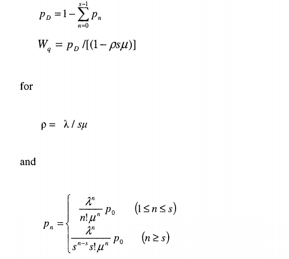
In the M/M/s (a.k.a. Erlang delay model), individuals arrive at a constant rate Poisson distribution and service duration has an exponential distribution, with average service time 1/μ, and there are s number of servers. Using this approach one can calculate the probability of a positive delay p_D and average delay W_D as:

Note that ρ is the average utilization for this queuing system and this system will only converge if ρ<1.

Extensions to the M/M/s model

Note that the M/M/s model can be adopted for additional complexity. For instance, priority queuing extensions can allow for preemptive (i.e., high priority patients displace current low-priority patients) or non-preemptive (i.e., high priority patients skip other patients in queue, but must wait for current low-priority patients being treated to have their treatment completed). M/M/s models can also allow for finite capacity where if the queue is already at its maximum, the patients must leave.

While the M/M/s model assumes the service time mean and variance are equal (as an exponential distribution is used), this assumption can be relaxed if one uses an alternative model such as M/G/1 or G/G/s. Applying these models, however, requires knowing both the mean and standard deviation of service duration.

Another extension would consider cases of time varying demand. For instance, hospital demand is highest during the day and after dinner compared to after midnight until early morning. One way to deal with this is to divide the workday into discrete periods. Then one can create a separate M/M/s model for each time period. This results in a stationary independent period-by-period (SIPP) model. SIPP models may be unreliable, however, if peak utilization occurs later than peak arrivals. However Lag SIPP models have been shown to help correct this issue (see Green et al. 2001)

Target utilization or delay

Some health care policymakers wish to target utilization. If utilization is too high, wait times will be high. If utilization is too low, however, this may appear inefficient. Targeting utilization, however, is not optimal. Larger facilities will be able to have higher utilization and achieve the same wait times compared to small facilities. Thus, if a service is characterized but lots of small capacity servers in a given geographic region, more capacity is needed. This is one reason why rural hospitals may complain that reimbursement is too low while policymakers believe that rural hospitals are inefficient; they are both right! Rural hospitals need to maintain more excess capacity to meet potential surges in demand compared to a large urban hospital.

Source:

• Green, Linda ” Queuing Analysis in Healthcare” in Patient Flow: Reducing Delays in Healthcare Delivery. 2013.